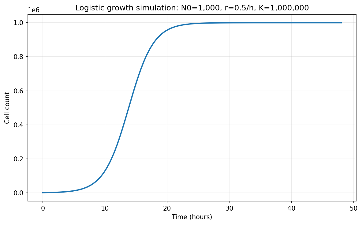
초기 세포 1,000개, 성장률 0.5/시간, 최대 수용량 100만 개인 로지스틱 성장을 파이썬으로 48시간 시뮬레이션하고, 시간에 따른 세포 수를 선 그래프로 그려 줘.
K
완료
실행 과정 8단계 · 33초
-
진행에이전트를 준비하고 있습니다.
-
진행질문에 맞는 도구와 데이터를 고르고 있습니다.
-
진행도구 11개, 데이터 0개, 라이브러리 5개를 골랐습니다.
-
계획요청은 로지스틱 성장 모델 \(dN/dt=rN(1-N/K)\)을 초기 세포수 1,000개, 성장률 0.5/시간, 최대 수용량 1,000,000개로 48시간 동안 시뮬레이션하고 선 그래프로 저장/제시하는 것입니다. 먼저 파이썬으로 수치 시뮬레이션을 수행하고 결과 CSV와 PNG 그래프를 현재 작업 디렉터리에 저장하겠습니다. 1. [ ] 로지스틱 성장 방정식과 파라미터를 정의한다. 2. [ ] 0–48시간 구간을 촘촘한 시간점으로 시뮬레이션한다. 3. [ ] 시간별 세포 수를 CSV 파일로 저장한다. 4. [ ] 시간에 따른 세포 수 선 그래프를 PNG 파일로 저장한다. 5. [ ] 생성된 파일과 핵심 결과를 사용자에게 요약한다.
-
코드 pythonpython
import numpy as np import pandas as pd import matplotlib.pyplot as plt from scipy.integrate import solve_ivp print("Step 1: Define logistic growth model and parameters") N0 = 1000 # initial cells r = 0.5 # per hour K = 1_000_000 # carrying capacity t_start, t_end = 0, 48 def logistic_growth(t, y): N = y[0] return [r * N * (1 - N / K)] print(f"Parameters: N0={N0}, r={r}/hour, K={K}, time={t_start}-{t_end} hours") print("\nStep 2: Simulate from 0 to 48 hours") t_eval = np.linspace(t_start, t_end, 481) # every 0.1 h sol = solve_ivp( logistic_growth, (t_start, t_end), [N0], t_eval=t_eval, method="RK45", rtol=1e-9, atol=1e-6 ) if not sol.success: raise RuntimeError(f"ODE solver failed: {sol.message}") time_h = sol.t cells = sol.y[0] print(f"Simulation completed with {len(time_h)} time points.") print(f"Final cell count at 48 h: {cells[-1]:,.0f}") print("\nStep 3: Save time-course table") df = pd.DataFrame({ "time_hours": time_h, "cell_count": cells }) csv_path = "logistic_growth_48h.csv" df.to_csv(csv_path, index=False) print(f"Saved CSV: {csv_path}") print("\nStep 4: Plot and save figure") plt.figure(figsize=(8, 5), dpi=150) plt.plot(time_h, cells, color="#1f77b4", linewidth=2) plt.xlabel("Time (hours)") plt.ylabel("Cell count") plt.title("Logistic growth simulation: N0=1,000, r=0.5/h, K=1,000,000") plt.grid(True, alpha=0.3) plt.tight_layout() png_path = "logistic_growth_48h.png" plt.savefig(png_path, bbox_inches="tight") plt.close() print(f"Saved plot: {png_path}") print("\nPreview of first and last rows:") print(pd.concat([df.head(), df.tail()]).to_string(index=False)) -
실행 결과
실행 결과 보기
Step 1: Define logistic growth model and parameters Parameters: N0=1000, r=0.5/hour, K=1000000, time=0-48 hours Step 2: Simulate from 0 to 48 hours Simulation completed with 481 time points. Final cell count at 48 h: 1,000,000 Step 3: Save time-course table Saved CSV: logistic_growth_48h.csv Step 4: Plot and save figure Plot saved to: logistic_growth_48h.png Saved plot: logistic_growth_48h.png Preview of first and last rows: time_hours cell_count 0.0 1000.000000 0.1 1051.217199 0.2 1105.054699 0.3 1161.646249 0.4 1221.132397 47.6 999999.953840 47.7 999999.956090 47.8 999999.958229 47.9 999999.960265 48.0 999999.962202 -
파일logistic_growth_48h.csv
-
파일logistic_growth_48h.png
시뮬레이션을 완료했습니다.
1. [✓] 로지스틱 성장 방정식과 파라미터를 정의했다.
2. [✓] 0–48시간 구간을 0.1시간 간격으로 시뮬레이션했다.
3. [✓] 시간별 세포 수를 CSV 파일로 저장했다.
4. [✓] 시간에 따른 세포 수 선 그래프를 PNG 파일로 저장했다.
5. [✓] 생성된 파일과 핵심 결과를 요약했다.
사용한 로지스틱 성장 모델은 다음과 같습니다.
\[
\frac{dN}{dt} = rN\left(1-\frac{N}{K}\right)
\]
파라미터:
- 초기 세포 수 \(N_0 = 1{,}000\)
- 성장률 \(r = 0.5/\text{시간}\)
- 최대 수용량 \(K = 1{,}000{,}000\)
- 시뮬레이션 시간: 0–48시간
결과:
- 48시간 후 세포 수: 약 999,999.96개
- 즉, 거의 최대 수용량인 1,000,000개에 도달했습니다.
생성된 파일:
- `logistic_growth_48h.csv`: 시간별 세포 수 데이터
- `logistic_growth_48h.png`: 시간에 따른 세포 수 선 그래프
초기 일부 결과 예시:
| 시간, h | 세포 수 |
|---:|---:|
| 0.0 | 1,000 |
| 0.1 | 1,051 |
| 0.2 | 1,105 |
| 0.3 | 1,162 |
| 0.4 | 1,221 |
48시간 부근 결과:
| 시간, h | 세포 수 |
|---:|---:|
| 47.6 | 999,999.95 |
| 47.7 | 999,999.96 |
| 47.8 | 999,999.96 |
| 47.9 | 999,999.96 |
| 48.0 | 999,999.96 |
그래프는 `logistic_growth_48h.png` 파일로 저장되어 다운로드할 수 있습니다.